50 Databricks Interview Questions that Data Engineers Come Across Often

k -

July 27, 2026

data engineering

Ace your databricks interview with expertly curated questions and in-depth, practical answers; covering everything from core Spark concepts to advanced Lakehouse architecture, performance optimization, security, and real-world implementation strategies.

1. What is Databricks and how it is not same as Apache Spark?

Databricks is a cloud-native, unified analytics platform designed for data engineering, data science, machine learning (ML), and business intelligence (BI). It was co-founded in 2013 by the original creators of Apache Spark — Matei Zaharia, Ali Ghodsi, and others — with the goal of simplifying large-scale data processing and accelerating the adoption of AI.

Databricks runs natively on major cloud providers (AWS, Microsoft Azure, and Google Cloud) and provides:

A collaborative notebook interface (with Python, SQL, Scala, R).
Fully managed compute clusters (including serverless options).
Integrated tools for ETL, streaming, ML lifecycle management (MLflow), data governance (Unity Catalog), and real-time dashboards.
Native support for Delta Lake, its open-source storage layer.

At its core, Databricks uses Apache Spark as its distributed compute engine, but it significantly extends, optimizes, and simplifies Spark for enterprise use.

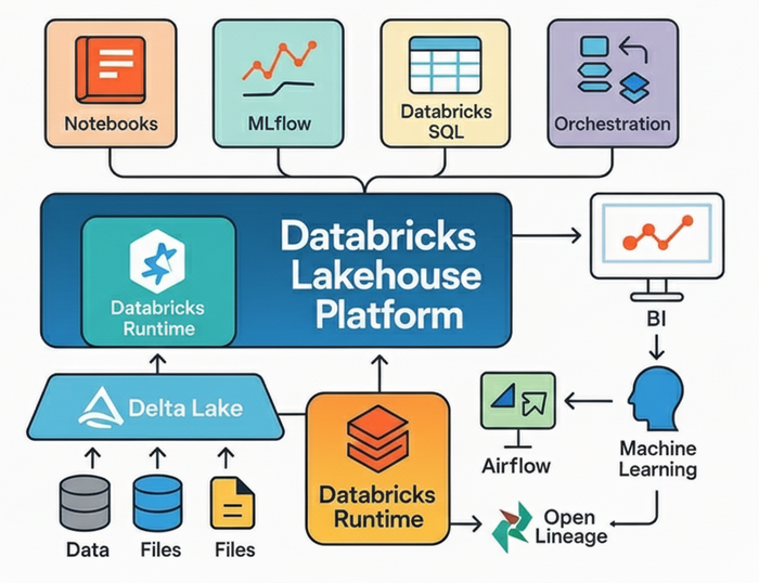
Key Differences Between Databricks and Apache Spark:

While Apache Spark is a foundational open-source framework, Databricks is a commercial, end-to-end platform built around Spark. Here’s a detailed comparison:

Nature

Apache Spark: Open-source distributed processing engine (Apache 2.0 license).

Databricks: Proprietary SaaS platform with open-core components (e.g., Delta Lake, MLflow).

Deployment & Management

Apache Spark: Requires manual setup: cluster configuration, resource tuning, monitoring, scaling, security, and patching.

Databricks: Fully managed: auto-scaling clusters, auto-termination, automatic updates, built-in monitoring, and cloud-native integration.

Performance

Apache Spark: Standard JVM-based execution. Optimizations (e.g., Catalyst optimizer, Tungsten) are good but generic.

Databricks: Includes Photon, a native vectorized query engine written in C++ that bypasses the JVM for SQL workloads — up to 10x faster than standard Spark. Also features Adaptive Query Execution (AQE) enhancements.

Storage Layer

Apache Spark: Works with raw file formats (Parquet, CSV, JSON) on HDFS, S3, etc. — no built-in transactional guarantees.

Databricks:Integrates Delta Lake by default — providing ACID transactions, schema enforcement, time travel, and upserts on data lakes.

User Experience

Apache Spark: Developers interact via APIs (PySpark, Scala) or command-line tools. No native UI for collaboration or job orchestration.

Databricks: Offers a unified workspace with collaborative notebooks, visual query editors, job schedulers, dashboards, and experiment tracking (via MLflow).

Security & Governance

Apache Spark: Requires manual integration with Kerberos, Ranger, or cloud IAM. No native data catalog or lineage.

Databricks: Provides Unity Catalog — a unified governance layer for fine-grained access control (row/column-level), data lineage, audit logging, and cross-cloud data sharing.

Streaming

Apache Spark: Structured Streaming is powerful but requires careful tuning for exactly-once semantics and state management.

Databricks: Enhanced streaming with Delta Live Tables (DLT) — a declarative framework for building reliable, testable, and maintainable data pipelines with automatic dependency resolution and monitoring.

Machine Learning

Apache Spark: MLlib provides basic algorithms, but model deployment, tracking, and CI/CD require custom tooling.

Databricks: Deep integration with MLflow for experiment tracking, model registry, and deployment. Also supports Feature Store, Model Serving, and LLM Playground for generative AI.

Cost & Operations

Apache Spark: Lower licensing cost (free), but higher operational overhead (DevOps, tuning, debugging).

Databricks: Higher per-hour compute cost, but reduced TCO due to automation, reliability, and developer productivity gains.

2. Explain the Delta Lake architecture in Databricks

Delta Lake is an open-source storage layer that brings ACID transactions, scalability, and reliability to data lakes. It is the default table format in Databricks and forms the backbone of the Lakehouse architecture.

Core Design Principles

Open Format: Built on Parquet (columnar storage) + transaction log (JSON/Parquet).
ACID Compliance: Ensures data integrity even with concurrent readers and writers.
Unified Batch + Streaming: Same table can be used for both batch and streaming workloads.
Time Travel: Query historical versions of data.
Schema Enforcement & Evolution: Prevent bad data and adapt to changing business needs.

Architectural Components

1. Data Files (Parquet)

Actual data is stored in Parquet format in cloud object storage (S3, ADLS, GCS).
Parquet provides columnar compression, predicate pushdown, and efficient I/O.

2. Transaction Log (`_delta_log`)

A hidden directory at the root of every Delta table: table_path/_delta_log/.
Records every change to the table as an ordered, immutable log.
Each transaction is written as:
A JSON file (for metadata, schema, actions like add, remove, txn).
Later compacted into Parquet checkpoint files (every 10 commits) for faster reads.
Actions logged:
add: New data file added.
remove: File deleted (e.g., during DELETE or compaction).
txn: Application-specific transaction identifier.
commitInfo: User, operation type, timestamp, etc.

3. ACID Transactions

Atomicity: A write either fully succeeds or fails — no partial writes.
Consistency: Schema validation ensures only conforming data is written.
Isolation: Readers see a consistent snapshot (via log versioning), even during concurrent writes.
Durability: Once committed, data is safely stored in cloud storage.

4. Optimizations

Data Skipping: Uses min/max statistics in Parquet footers + Delta log to skip irrelevant files.
Z-Ordering: Physically co-locates related data (e.g., country = 'US' and state = 'CA') to improve multi-column query performance.
Compaction (OPTIMIZE): Merges small files into larger ones (e.g., 1 GB) to reduce metadata overhead.
Vacuum: Removes old files no longer referenced by the log (default retention: 7 days).

5. Time Travel (Versioning)

Every write increments the table version.
Query any historical version:

SELECT * FROM my_table VERSION AS OF 5;
SELECT * FROM my_table TIMESTAMP AS OF '2024-06-01 10:00:00';

Enables auditing, rollback, and reproducible ML experiments.

6. Streaming Integration

Delta tables can be sources and sinks for Spark Structured Streaming.
Supports exactly-once processing via idempotent writes and offset tracking.

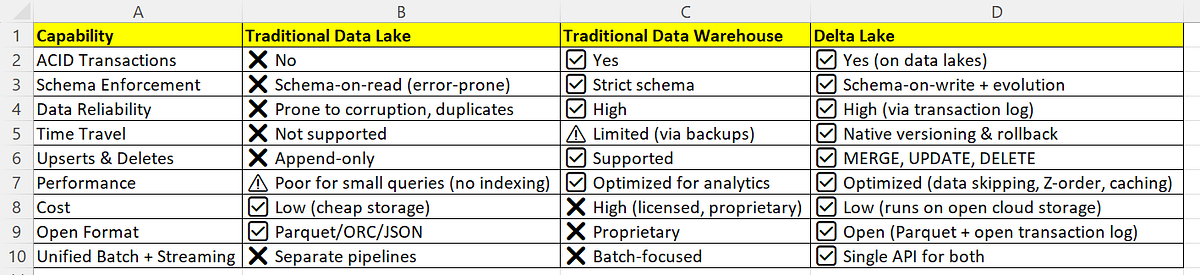
3. List the advantages of Delta Lake over traditional data lake and data warehouse?

Delta Lake bridges the gap between data lakes (cheap, flexible, unstructured) and data warehouses (reliable, structured, expensive).

4. What is new from Databricks Runtime 15 and what are it’s Latest Features?

Databricks Runtime (DBR) 15.0, released in Q1 2024, is a major leap forward in performance, AI, and serverless capabilities. It’s built on Apache Spark 3.5 and includes significant proprietary enhancements. Key Innovations in DBR 15:

1. Photon Engine 3.0

Vectorized C++ execution for SQL and DataFrame workloads.
3–10x faster than standard Spark for complex queries (e.g., joins, aggregations).
Full support for nested types (structs, arrays), geospatial functions, and ANSI SQL compliance.

2. Serverless Compute

No cluster management: Databricks automatically provisions and scales compute.
Per-second billing, automatic patching, and zero maintenance.
Ideal for SQL analytics, notebooks, and jobs with variable workloads.

3. Delta Lake 3.0 Integration

Faster MERGE operations with improved concurrency control.
Extended time travel: Retention up to 365 days (vs. 30 days previously).
Delta Sharing 2.0: Secure, cross-organization data sharing without copying.

4. AI & Generative AI Enhancements

Databricks LLM Playground: Test and compare foundation models (Llama 2, Mistral, Databricks DBRX).
Vector Search: Native support for semantic search and RAG (Retrieval-Augmented Generation).
MLflow 2.10: Improved model registry, drift detection, and LLM evaluation metrics.

5. Unity Catalog Upgrades

Row- and column-level security enforced at query runtime.
Cross-workspace data sharing with fine-grained permissions.
Data lineage from source to dashboard.

6. Delta Live Tables (DLT) Improvements

Declarative pipeline testing: Define expectations (expectations) to validate data quality.
Auto-scaling and failure recovery with detailed observability.

7. Language & Library Support

Python 3.11 as default.
Pre-installed: PyTorch 2.1, TensorFlow 2.14, scikit-learn 1.4, Hugging Face Transformers.

8. Security & Compliance

FIPS 140–2 compliance for government/regulated workloads.
PrivateLink support for secure network isolation.

5. Explain Delta Lakes schema evolution capability.

Schema evolution is Delta Lake’s ability to safely modify a table’s structure over time while maintaining data integrity and backward compatibility. This is critical in agile environments where data models change frequently.

Business needs evolve (e.g., new user attributes, IoT sensor fields).
Without evolution, you’d need to:
Recreate tables.
Rewrite historical data.
Break existing pipelines.

Delta Lake solves this with controlled, explicit schema changes.

Schema Evolution Workongs

1. Schema Enforcement (Default Behavior)

Delta Lake rejects writes that don’t match the current schema.
Prevents accidental data corruption (e.g., writing a string to an integer column).

2. Enabling Schema Evolution

Use write options to allow schema changes:

mergeSchema = true: Add new columns; preserve existing data.
overwriteSchema = true: Replace the entire schema (use with caution).

Example (PySpark):

# Add new columns to an existing Delta table
new_data.write.format("delta") \
    .mode("append") \
    .option("mergeSchema", "true") \
    .save("/mnt/delta/user_table")

Example (SQL):

-- Databricks SQL supports automatic schema evolution in some contexts
CREATE OR REPLACE TABLE user_table
AS SELECT user_id, name, email, signup_date FROM new_source;

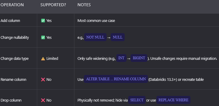
3. Supported Schema Changes

4. Backward & Forward Compatibility

Old data: New columns appear as NULL.
Old queries: Continue to work (ignore new columns).
New queries: Can access all columns.

5. Real-World Example

v1: Table has user_id, name.
v2: Add email and country.
With mergeSchema=true:
Records written in v1: email = NULL, country = NULL.
Records written in v2: full data.
Query: SELECT user_id, email FROM table → works for all records.

6. Best Practices

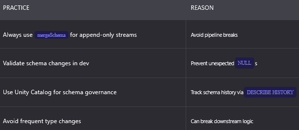
Always explicitly enable schema evolution (mergeSchema).
Avoid frequent schema changes — design for extensibility.
Use Delta’s DESCRIBE HISTORY to track schema changes over time.
Test schema changes in non-production environments.

6. How is security managed in Databricks at the workspace and cluster level?

Security in Databricks is implemented through a defense-in-depth strategy, with granular controls at both the workspace (platform) and cluster (compute) levels. The model integrates with cloud-native identity providers and enforces least-privilege access.

A. Workspace-Level Security

The workspace is the top-level container for users, notebooks, jobs, clusters, and data assets. Security here governs who can do what across the entire environment.

1. Identity & Access Management (IAM)

Cloud Identity Federation: Databricks integrates with:
Azure AD (via SAML or SCIM)
AWS IAM Identity Center (formerly SSO)
Google Cloud Identity
Single Sign-On (SSO): Users log in via corporate credentials — no local Databricks passwords.
SCIM Provisioning: Automates user/group provisioning and deprovisioning from identity providers.

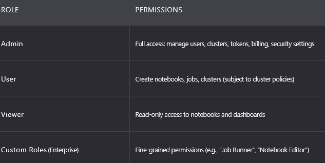
2. Role-Based Access Control (RBAC)

Databricks uses workspace-level roles to define permissions:

3. Network Security

Private Network Connectivity:
Azure: VNet injection, Private Link
AWS: VPC peering, PrivateLink, customer-managed VPC
GCP: VPC SC, private service connect
IP Access Lists: Restrict workspace login to corporate IP ranges.
Data Exfiltration Prevention: Disable public internet access to clusters; force traffic through private endpoints.

4. Audit Logging & Monitoring

Audit Logs: Captured in cloud storage (S3, ADLS, GCS) for all admin actions (user logins, cluster creation, permission changes).
Integration with SIEM: Logs can be streamed to Splunk, Datadog, or Azure Sentinel.

B. Cluster-Level Security

Clusters are ephemeral compute resources that execute code. Security here ensures isolation, credential management, and secure data access.

1. Cluster Access Control

Only users with “Can Manage” or “Can Restart” permissions can interact with a cluster.
Cluster Policies: Enforce security standards (e.g., “must use FIPS-compliant images”, “must disable public IPs”).

2. Credential Passthrough (High Concurrency Clusters)

Purpose: Allow users to access cloud storage (e.g., S3, ADLS) using their own IAM/AD credentials — not cluster-level credentials.
How it works:
On Azure: Azure AD passthrough maps user identity to Azure RBAC roles on storage.
On AWS: IAM roles for service accounts (IRSA) or instance profiles mapped via SAML.
Benefit: Enforces row/column-level security at the storage layer; no shared credentials.

3. Secure Secret Management

Databricks Secrets: Store tokens, passwords, API keys in scoped secret backends:
Databricks-backed (managed)
Azure Key Vault, AWS Secrets Manager, HashiCorp Vault

Accessed in notebooks via:

dbutils.secrets.get(scope="prod", key="snowflake-pwd")

Secrets are never exposed in logs or UI.

4. Isolation & Sandboxing

Standard Clusters: Shared by a user or team — code runs with user identity.
High Concurrency Clusters: Multi-tenant, with fine-grained isolation between users (via containerization and credential passthrough).
Job-Only Clusters: Ephemeral, auto-terminated after job completion — minimizes attack surface.

5. Encryption

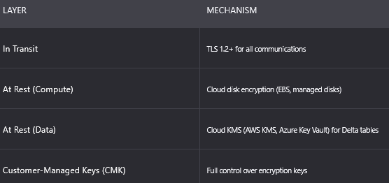
In Transit: TLS 1.2+ for all communications.
At Rest:
Managed: Databricks encrypts notebooks, job configs, etc., using cloud KMS (e.g., AWS KMS, Azure Key Vault).
Customer-Managed Keys (CMK): Full control over encryption keys for data and metadata.

7. Explain Unity Catalog and its role.

Unity Catalog is Databricks’ unified governance solution for data and AI assets across clouds, workspaces, and regions. It brings enterprise-grade security, discovery, and lineage to the Lakehouse.

Core Architecture

Unity Catalog introduces a three-level namespace:

<metastore>.<catalog>.<schema>.<table>

Key Capabilities

1. Fine-Grained Access Control

Permissions model: Similar to SQL databases (SELECT, MODIFY, OWN, EXECUTE).
Grants at any level: Catalog, schema, table, column, or row.
Example:

GRANT SELECT (ssn, salary) ON TABLE hr.employees TO ROLE finance_analyst;
GRANT SELECT ON TABLE hr.employees TO ROLE hr_staff;
CREATE FUNCTION mask_ssn() ... ;

2. Row-Level Security (RLS)

Use dynamic views or row filter functions:

CREATE ROW FILTER hr.employee_filter
ON hr.employees
USING (region = current_user_region());

Enforced at query runtime — transparent to users.

3. Data Lineage & Impact Analysis

Automatically tracks:
Column-level lineage (from source files → ETL → dashboard).
Downstream impact: “If I change this column, which reports break?”
Visualized in the Data Explorer UI.

4. Audit & Compliance

All data access logged (who queried what, when).
Integration with audit logs and cloud trails.

5. Cross-Cloud & Cross-Workspace Sharing

Delta Sharing: Share live tables with external organizations without copying data.
Internal Sharing: Grant access to tables across workspaces in the same account.

6. Unified Metadata

Replaces legacy Hive metastore.
Supports tables, views, functions, volumes (for unstructured data), and models.

8. What is the purpose of Databricks Repos?

Databricks Repos is a native Git integration that enables version control, CI/CD, and collaboration for notebooks and code directly within the Databricks workspace.

Before Repos, the users:

Downloaded notebooks as .dbc files (binary, not diff-friendly).
Used external IDEs with Databricks Connect (complex setup).
Lacked branching, pull requests, or audit trails.

Repos solves this by bringing Git workflows into Databricks.

Key Features & Workflow

1. Git Integration

Connect to GitHub, GitLab, Azure DevOps, Bitbucket.
Clone a repo directly into a workspace folder.

2. Notebook-as-Code

Notebooks are stored as .py, .sql, .scala, or .r files (not JSON).
Enables line-by-line diffs, code reviews, and IDE compatibility.

3. Branching & Merging

Switch branches directly in the UI.
Make changes → commit → push → create pull request (in Git provider).
No local setup required.

4. CI/CD Integration

Trigger Databricks Jobs on Git push (via webhooks).
Use Databricks CLI or Workflows API in CI pipelines to:
Deploy notebooks
Run tests
Promote models

5. Collaboration & Audit

Full Git history visible in Databricks.
See who changed what and when.

9. How does Databricks support multi-cloud and hybrid cloud deployments?

Databricks is cloud-agnostic by design, supporting multi-cloud, hybrid, and multi-region architectures.

A. Multi-Cloud Support

Single Control Plane: Manage workspaces on AWS, Azure, and GCP from one account console.
Consistent Experience: Same UI, APIs, and features across clouds.
Use Cases:
Cloud bursting: Run workloads on the cheapest cloud.
Vendor diversification: Avoid lock-in.
Regional compliance: Store EU data in Azure (Frankfurt), US data in AWS (us-east-1).

B. Hybrid Cloud (On-Prem + Cloud)

While Databricks is cloud-native, hybrid scenarios are supported via:

1. Databricks on AWS/Azure with On-Prem Data Sources

Use Databricks Connect or Partner Connectors (e.g., JDBC/ODBC) to read from on-prem databases.
Not recommended for large-scale ETL (network latency, egress costs).

2. Delta Sharing for Hybrid

Share data from cloud-based Delta tables with on-prem consumers via open protocol (no Databricks license needed for recipient).

3. Limited On-Prem Option

Databricks Runtime for Docker: Run Spark jobs in on-prem Kubernetes (experimental, not full platform).
No native on-prem Databricks workspace — the platform is SaaS-only.

C. Multi-Region & Disaster Recovery

Workspaces: Deploy in multiple regions for latency/compliance.
Unity Catalog: Replicate metastore across regions (preview).
Delta Lake: Tables are cloud-storage-native — copy via DistCp or cloud replication.

10. Describe ML pipelines and MLflow in Databricks.

Databricks provides a unified MLOps platform centered around MLflow — an open-source project co-created by Databricks.

A. MLflow: The Open MLOps Platform

MLflow standardizes the ML lifecycle across four components:

1. MLflow Tracking

Log parameters, metrics, code version, and artifacts (models, plots) from any environment.
In Databricks: Auto-logged for every notebook run.
UI shows experiment comparisons, model performance trends.

2. MLflow Models

Standard format to package models with:
Code
Dependencies
Inference logic (predict() function)
Supports multiple flavors: Python function, PyTorch, TensorFlow, sklearn, custom.

3. MLflow Model Registry

Centralized model store with:
Versioning
Staging (Staging → Production)
Annotations & descriptions
Webhooks for CI/CD
Governed by Unity Catalog (in newer versions).

4. MLflow Projects

Package ML code as reproducible projects (with MLproject file).
Run locally, on Databricks, or in Docker.

B. ML Pipelines in Databricks

Databricks enhances MLflow with native integrations:

1. AutoML

Point-and-click UI to auto-train models on a dataset.
Generates Python notebook with full MLflow tracking.

2. Feature Store

Central catalog of curated features.
Ensures training-serving consistency.
Integrated with Delta Lake and Unity Catalog.

3. Model Serving

Deploy models as REST endpoints (real-time) or batch jobs.
Auto-scaling, monitoring, and A/B testing.

4. Workflows (Jobs) for Orchestration

Schedule end-to-end ML pipelines:

5. LLM & Generative AI Support

Databricks Model Serving supports open LLMs (Llama, Mistral).
Vector Search for RAG applications.
MLflow 2.10+: Native LLM evaluation metrics (toxicity, relevance).

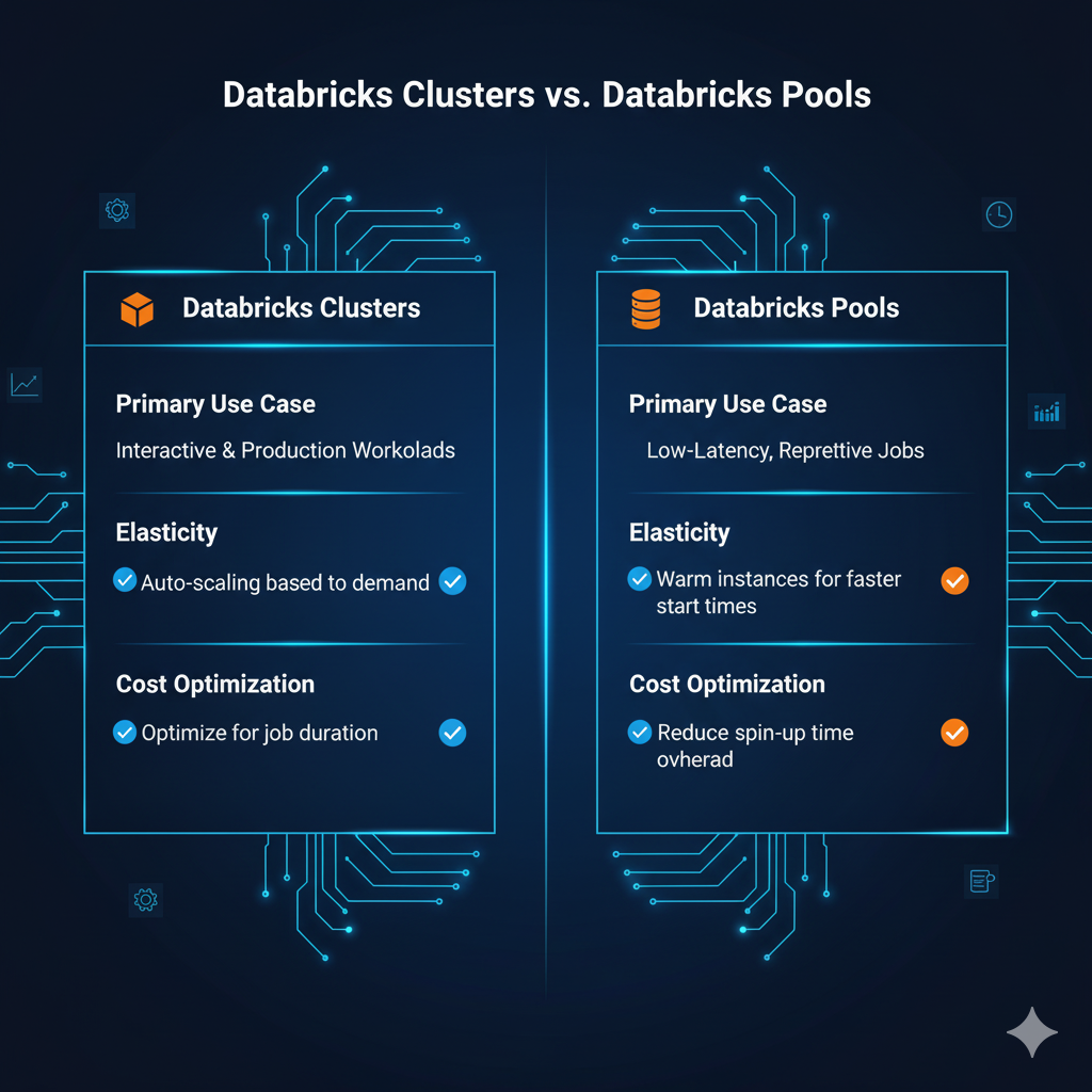
11. What is the difference between a Databricks cluster and a pool?

Purpose

Databricks Cluster: Compute environment to execute code (notebooks, jobs, streaming).

Databricks Instance Pool: Pre-warmed reserve of VM instances to accelerate cluster startup.

Lifecycle

Databricks Cluster: Created on-demand; terminated when idle (or manually).

Databricks Instance Pool: Long-running; persists across cluster lifecycles.

Resource Type

Databricks Cluster: Logical grouping of compute + configuration (runtime, libraries, autoscaling).

Databricks Instance Pool: Physical VM instances in the cloud (EC2, Azure VMs, GCE).

Billing

Databricks Cluster: Billed per second while running (includes cloud + DBU costs).

Databricks Instance Pool: Billed per second while provisioned (even if idle) — only cloud cost (no DBUs).

Use Case

Databricks Cluster: Running actual workloads (ETL, ML, SQL).

Databricks Instance Pool: Reducing startup latency for interactive or frequent job clusters.

When you create a cluster, Databricks normally:

Requests VMs from the cloud provider.
Waits for OS boot, Databricks runtime installation (~3–8 minutes).
Starts the Spark driver/executor processes.

With an Instance Pool:

A pool of pre-initialized VMs (with Databricks runtime pre-installed) sits ready.
When a cluster is created, it pulls instances from the pool.
Cluster startup drops to ~1–2 minutes (no OS/runtime setup needed).

Instance Pool Features

Pre-warmed Instances: VMs are launched with Databricks runtime, but no Spark context.
Auto-scaling: Pools can scale out/in based on demand (min/max size).
Spot Instance Support: Use low-cost spot instances in pools (with fallback to on-demand).
Isolation: Pools can be dedicated to specific users, workloads, or node types (e.g., GPU pools for ML).
Cost Trade-off: You pay for idle pool instances, but save on developer time and job latency.

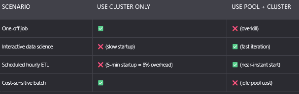
When to Use What

12. How does Databricks optimize Spark for performance?

Databricks doesn’t just run Apache Spark. It re-engineers and extends it for cloud-scale performance. Key optimizations span query execution, I/O, memory, and concurrency.

A. Photon Engine: Native Vectorized Execution

What it is: A C++-based query engine that bypasses the JVM for SQL/DataFrame workloads.

How it works:

Compiles Spark Catalyst plans into native machine code.
Uses SIMD (Single Instruction, Multiple Data) for vectorized processing.
Integrates with cloud storage APIs for zero-copy I/O.

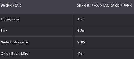
Performance Gains: 3–10x faster than standard Spark for:

Complex joins
Aggregations
Nested data (structs, arrays)
Geospatial functions

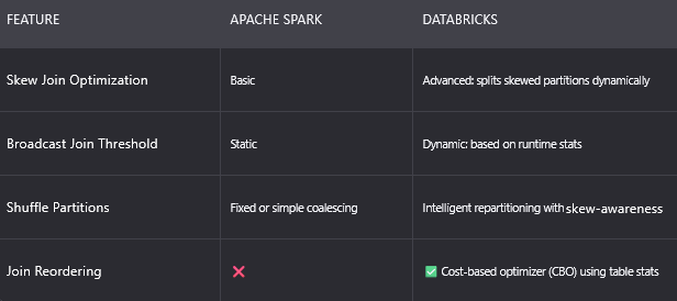
B. Adaptive Query Execution (AQE) Enhancements

While Apache Spark introduced AQE in 3.0, Databricks extends it significantly:

C. I/O and Storage Optimizations

1. Delta Lake Integration

Data Skipping: Uses min/max statistics in Parquet footers + Delta log to skip irrelevant files.
Z-Ordering: Physically co-locates related data (e.g., country + city) to improve multi-predicate queries.
Caching: Automatically caches hot data in cluster SSDs (via Delta Cache).

2. Cloud-Native I/O

Direct S3/ADLS/GCS Access: Bypasses HDFS; uses cloud-optimized connectors.
Concurrent I/O: Hundreds of threads per executor for high-throughput reads.

D. Memory & CPU Efficiency

Off-Heap Memory Management: Reduces GC pauses via Tungsten (shared with Spark) + Photon enhancements.
Columnar Processing: Keeps data in columnar format in memory (not row-based) for analytical workloads.
GPU Acceleration: Supports RAPIDS for GPU-accelerated Spark (on GPU clusters).

E. Concurrency & Isolation

High Concurrency Clusters: Use containerization to isolate user workloads on shared clusters.
Fair Scheduling: Built-in support for multi-tenant resource sharing.

13. How are jobs managed in Databricks?

Databricks Jobs are the primary mechanism for production orchestration of notebooks, JARs, Python scripts, or Delta Live Tables pipelines.

A Job consists of:

Task(s): Unit of work (notebook, JAR, Python file, etc.).
Cluster Specification: New job cluster, existing cluster, or instance pool.
Schedule: Cron-based or triggered via API/webhook.
Dependencies: Task ordering (linear or DAG).
Notifications: Email, Slack, or webhook on success/failure.

Key Features

1. Job Clusters vs. Interactive Clusters

Job Cluster:

Created per job run.
Auto-terminated after completion.
Isolated (no interference from other users).
Recommended for production.

Interactive Cluster:

Shared, long-running.
Risk of resource contention.
Only for development/testing.

2. Multi-Task Jobs (DAG Support)

Define dependencies between tasks:

# Task A → Task B (only if A succeeds)
# Task A → Task C (runs in parallel with B)

Visual DAG editor in UI.

3. Parameterization

Pass parameters to notebooks/scripts (see Q14).
Use widgets for dynamic input.

4. Monitoring & Debugging

Run History: View logs, metrics, Spark UI for every run.
Alerts: Configure on failure, duration, or custom conditions.
Retry Policy: Auto-retry on transient failures (with exponential backoff).

5. CI/CD Integration

Deploy jobs via Databricks CLI, Terraform, or REST API.
Store job definitions in Git (via Repos).

6. Serverless Jobs (DBR 13+)

No cluster management: Databricks auto-provisions compute.
Pay per task duration (not cluster uptime).
Ideal for lightweight, infrequent jobs.

14. How to parameterize notebooks in Databricks?

Parameterization enables reusable, dynamic notebooks — critical for CI/CD, testing, and multi-environment deployments.

Methods of Parameterization

1. Widgets (Interactive & Job Runs)

Create widget in notebook:

dbutils.widgets.text("input_path", "/default/path", "Input Path")
dbutils.widgets.dropdown("env", "dev", ["dev", "prod"], "Environment")

Read value:

input_path = dbutils.widgets.get("input_path")
env = dbutils.widgets.get("env")

In Jobs: Pass parameters via UI or API:

{ "input_path": "/prod/data", "env": "prod" }

2. Context Parameters (Jobs Only)

Use %run with arguments (limited support).
Better: Use Python/Scala scripts instead of notebooks for pure parameterization.

3. Environment Variables (Advanced)

Set via cluster init scripts or job environment variables.

Access in Python:

import os
env = os.getenv("ENV", "dev")

4. Delta Live Tables (DLT) Parameters

Special syntax for DLT pipelines:

@dlt.table
def sales():
    return spark.read.csv(spark.conf.get("mypipeline.input"))

Pass via pipeline settings:

{ "mypipeline.input": "s3://prod/sales" }

Use widgets for most notebook-based workflows.
Validate inputs:

assert env in ["dev", "prod"], "Invalid environment"

15. What is Auto Loader in Databricks?

Auto Loader is a streaming data ingestion service that incrementally and efficiently loads new files from cloud storage (S3, ADLS, GCS) into Delta Lake — without requiring complex file listing or watermarking.

Why Auto Loader? The Problem It Solves

Traditional file ingestion challenges:

Listing millions of files is slow and expensive (cloud API costs).
Exactly-once processing is hard (files can arrive late or be updated).
Schema inference for heterogeneous data is manual.

Auto Loader solves these with two modes:

A. Directory Listing Mode (Default)

Uses cloud storage notifications (e.g., S3 Event Notifications, Azure Event Grid) to track new files.
Maintains an internal offset log to avoid reprocessing.

Requirements:

Cloud event notifications configured (Databricks can auto-configure via UI).

Use Case: High-volume, continuous ingestion (e.g., IoT, logs).

df = spark.readStream.format("cloudFiles") \
  .option("cloudFiles.format", "json") \
  .option("cloudFiles.schemaLocation", "/schema") \
  .load("s3://my-bucket/events/")

df.writeStream.format("delta") \
  .option("checkpointLocation", "/checkpoints") \
  .table("events_raw")

B. File Notification Mode (Legacy)

Uses manual file listing (slower, but no cloud setup needed).
Only for small-scale or restricted environments.

Key Features

1. Automatic Schema Inference & Evolution

Infers schema from first batch of files.
Evolves schema as new fields appear (uses Delta Lake’s mergeSchema).

2. Exactly-Once Semantics

Guarantees no duplicates, even with:
Late-arriving files
Job restarts
Duplicate cloud notifications

3. Optimized File Discovery

Avoids full directory scans — uses event-driven triggers.
Scales to billions of files.

4. Structured Streaming Integration

Output is a Structured Streaming DataFrame — can be:
Written to Delta Lake
Joined with static data
Aggregated in real time

5. Rescanning for Late Data

Supports rescanning of historical partitions if late data arrives.

Use Cases

Log ingestion (application, security, network)
IoT telemetry (sensor data from devices)
Clickstream analytics
CDC (Change Data Capture) from databases

16. How are streaming and batch processing unified in Databricks?

Databricks achieves true unification of batch and streaming through a combination of Delta Lake, Apache Spark Structured Streaming, and declarative pipeline frameworks like Delta Live Tables (DLT). This eliminates the historical need for separate systems (Lambda/Kappa architectures).

Core Principles of Unification

Single Storage Layer: Delta Lake tables serve as both batch sources/sinks and streaming sources/sinks. No data duplication.

Single Compute Engine: Apache Spark (enhanced by Databricks) processes both batch (spark.read) and streaming (spark.readStream) workloads with the same API.

Single Programming Model: Developers write identical DataFrame/SQL logic — only the trigger (batch vs. continuous) differs.

Single Governance Layer: Unity Catalog applies consistent security, lineage, and auditing across batch and streaming jobs.

Technical Implementation

1. Delta Lake as the Unified Table Format

A Delta table can be:
Read in batch: spark.read.table("events")
Read as a stream: spark.readStream.table("events")
Written in batch: df.write.saveAsTable("aggregates")
Written as a stream: df.writeStream.trigger(processingTime='1 minute').table("aggregates")
Exactly-once semantics are guaranteed for both via Delta’s ACID transactions and idempotent writes.

2. Structured Streaming with Continuous Processing

Micro-batch mode (default): Processes data in small batches (e.g., every 1–10 seconds).
Continuous mode (low-latency): Sub-second processing (experimental, for simple operations).
Checkpointing: Maintains offsets and state in cloud storage for fault tolerance.

3. Delta Live Tables (DLT): Declarative Unification

DLT is Databricks’ declarative framework for building reliable, testable, and maintainable data pipelines that work identically for batch and streaming.

Declarative Syntax:

@dlt.table
def sales_raw():
    return (
        spark.readStream  # or spark.read for batch replay
          .format("cloudFiles")
          .option("cloudFiles.format", "json")
          .load("/raw/sales")
    )

@dlt.table
def sales_clean():
    return dlt.read("sales_raw").filter(col("amount") > 0)

Automatic Orchestration:

DLT infers dependencies and builds a DAG.
Same pipeline runs in continuous streaming mode or batch backfill mode.
Data Quality Enforcement:

@dlt.expect("valid_user_id", "user_id IS NOT NULL")
def users_clean():
    return dlt.read("users_raw")

4. Time Travel for Backfill & Replay

Delta Time Travel can be used to reprocess historical data as a batch job using the same streaming logic:

CREATE OR REPLACE TEMP VIEW historical_events AS
SELECT * FROM events VERSION AS OF 100;

-- Apply same transformation logic used in streaming
INSERT INTO aggregates SELECT count(*) FROM historical_events;

17. What are best practices for cost management in Databricks?

Cost optimization in Databricks requires managing compute (clusters), storage, and licensing (DBUs). Below are enterprise-proven strategies.

A. Compute Optimization

1. Use Auto-Termination

Set auto-terminate (e.g., 10–20 mins) on interactive clusters to avoid idle costs.
Job clusters auto-terminate by default — always prefer them for production.

2. Leverage Instance Pools

For frequent/interactive workloads, use instance pools to reduce startup time and improve developer productivity — but monitor idle pool costs.

3. Right-Size Clusters

Avoid over-provisioning: Use cluster logs and Spark UI to analyze CPU/memory usage.
Use Photon: Faster execution = shorter runtime = lower cost.
Spot Instances: Use preemptible VMs (up to 60–90% discount) for fault-tolerant workloads (e.g., ETL, ML training).

4. Serverless Compute (DBR 13+)

Databricks SQL Serverless: Pay per query — no cluster management.
Serverless Jobs: Ideal for lightweight, infrequent tasks.

B. Storage Optimization

1. Optimize Delta Tables

Run OPTIMIZE regularly to merge small files (reduces metadata overhead).
Use Z-ORDER on high-cardinality filter columns to reduce I/O.
VACUUM old files (default 7-day retention) to reduce storage costs.

2. Tiered Storage

Move cold data to low-cost storage tiers (e.g., S3 Glacier, Azure Cool Blob).
Use Delta Sharing instead of copying data for external consumers.

C. Licensing & DBU Management

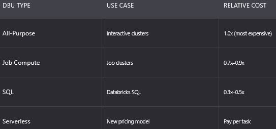
1. Understand DBU Types

All-Purpose DBUs: For interactive clusters (most expensive).
Job Compute DBUs: For job clusters (discounted).
SQL DBUs: For Databricks SQL (lowest cost).
Serverless DBUs: New pricing model (pay per task/query).

2. Monitor Usage

Use Account Console → Usage to track DBU consumption by workspace, user, or workload.
Set budget alerts via cloud provider (AWS Cost Explorer, Azure Cost Management).

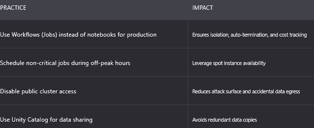
D. Operational Best Practices

18. How do you debug Databricks SQL or Spark queries?

Debugging in Databricks leverages built-in UIs, logs, and Spark-native tooling.

A. For Databricks SQL Queries

1. Query History (SQL Console)

View execution time, bytes scanned, rows returned.
Click into a query to see:
Query plan (logical + physical)
Execution details (stages, tasks, shuffle read/write)
Error messages (with line numbers)

2. Explain Plans

Use EXPLAIN to see optimization:

EXPLAIN EXTENDED SELECT * FROM sales WHERE region = 'EU';

Look for:

Data skipping (files skipped due to stats)
Broadcast joins (efficient for small tables)
Skew (uneven task durations)

3. Query Profile (Photon)

Visual breakdown of CPU time, I/O wait, memory usage per operator.

B. For Spark (PySpark/Scala) Queries

1. Spark UI (Accessible from Notebook or Job Run)

Jobs Tab: See DAG, stage duration, task distribution.
Stages Tab: Identify stragglers, skew, GC overhead.
Storage Tab: Check if RDDs/DataFrames are cached effectively.
SQL Tab: View physical plans for DataFrame operations.

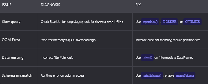
2. Common Debugging Scenarios

3. Logging & Print Statements

In notebooks:

print("Row count:", df.count())  # Caution: action triggers job
df.filter(...).explain()         # Shows plan without execution

Use display() for sample data inspection.

4. Delta Lake-Specific Debugging

DESCRIBE HISTORY table: See schema changes, operation types.
DESCRIBE DETAIL table: View file stats, partitioning, size.

19. How does Databricks handle secrets management?

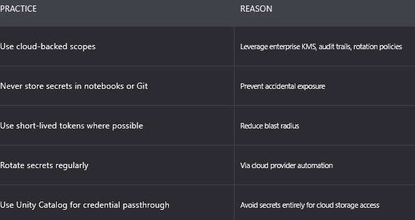
Databricks provides secure, centralized secret management to avoid hardcoding credentials in notebooks or jobs.

A. Databricks Secrets Backend

1. Secret Scopes

Logical containers for secrets (e.g., prod-db, aws-keys).
Two types:
Databricks-backed: Managed by Databricks (encrypted at rest).
Cloud-backed: Integrated with:
Azure Key Vault
AWS Secrets Manager
HashiCorp Vault

2. Creating & Accessing Secrets

Create via CLI:

databricks secrets create-scope --scope prod
databricks secrets put --scope prod --key snowflake-pwd

Access in Notebook:

pwd = dbutils.secrets.get(scope="prod", key="snowflake-pwd")

Never appears in logs, UI, or cell output.

3. Access Control

Permissions per scope:

MANAGE: Create/delete secrets
READ: Retrieve secrets
Managed via workspace admin console or Unity Catalog (in newer versions).

20. Describe the difference between batch and streaming processing in Databricks.

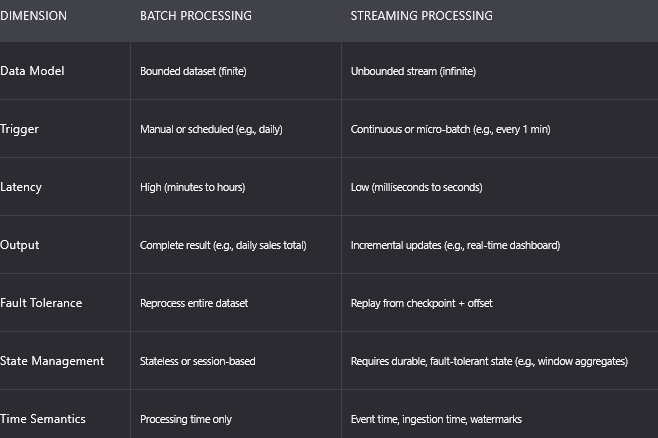
While Databricks unifies the programming model, batch and streaming remain distinct execution paradigms with different characteristics.

Implementation in Databricks

Batch

# Read full table
df = spark.read.table("raw_events")
# Transform
clean = df.filter(col("status") == "success")
# Write once
clean.write.mode("overwrite").saveAsTable("clean_events")

Runs to completion.
No state retained after job ends.

Streaming

# Read stream
stream = spark.readStream.table("raw_events")
# Transform with state (e.g., window)
windowed = stream.groupBy(
    window("event_time", "10 minutes"), "user_id"
).count()
# Write continuously
query = windowed.writeStream \
    .trigger(processingTime='1 minute') \
    .option("checkpointLocation", "/chkpt") \
    .table("user_activity_10min")
query.awaitTermination()

Runs indefinitely.
Maintains state (e.g., window counts) in checkpoint location.
Uses watermarks to handle late data.

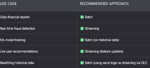
When to Use Which?

21. What is Z-Ordering and how does it improve query performance?

Z-Ordering (also known as Z-order curve clustering) is a data layout optimization technique in Delta Lake that physically co-locates related data on disk to dramatically improve multi-column predicate query performance.

Unlike traditional range partitioning (which only optimizes for one or two columns), Z-Ordering uses a space-filling curve to interleave multiple columns into a single sort order — minimizing I/O for queries that filter on any combination of those columns.

1. The Problem with Naive Layouts

In a standard Parquet file:
Data is stored in row groups.
Without clustering, records with country = 'US' and device = 'mobile' may be scattered across hundreds of files.

A query like:

SELECT * FROM events WHERE country = 'US' AND device = 'mobile'

must scan all files, even if only 0.1% match.

2. Z-Order Curve Mechanics

Z-Ordering maps multi-dimensional data (e.g., (country, device, event_type)) into a 1D space-filling curve.
It interleaves bits of each column’s value to create a composite sort key.
Example: For two columns A (binary: 101) and B (binary: 011), the Z-value is 1 0 0 1 1 1.
Data is then sorted by this Z-value and written to Parquet files.

3. Resulting Data Layout

Records with similar values across multiple dimensions are stored in the same or adjacent files.
Enables data skipping at the file level using min/max statistics in Parquet footers.

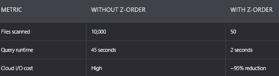
Implementation in Databricks

-- Z-Order on multiple columns
OPTIMIZE events_table ZORDER BY (country, device, event_type);

Key Considerations

Cost: OPTIMIZE is a write-intensive operation—run during off-peak hours.
Diminishing Returns: Avoid Z-Ordering on >4 columns (curve becomes less effective).
Partitioning First: Always partition by high-cardinality, low-selectivity columns (e.g., date) before Z-Ordering.

Monitoring Effectiveness

Use Delta Lake’s file statistics:

DESCRIBE DETAIL events;

Check Spark UI for “number of files read” before/after.

22. What is Auto Termination on clusters?

Auto Termination is a cluster lifecycle management feature that automatically shuts down a Databricks cluster after a specified period of inactivity (no commands executed).

Inactivity Timer: Starts when the last command (notebook cell, job, SQL query) finishes.

Default:

Interactive clusters: 120 minutes (configurable from 1–10,000 minutes).
Job clusters: Always auto-terminate after job completion (not configurable).
Graceful Shutdown:
Saves notebook state.
Terminates all executors and driver.
Releases cloud VMs (stops billing).

Best Practices

Set Aggressive Timeouts:

Interactive clusters: 15–30 minutes for most teams.
Shared clusters: 10 minutes to encourage job cluster usage.

Use Job Clusters for Production:

They auto-terminate by design — no configuration needed.

Combine with Cluster Policies:

Enforce auto-termination via cluster policy:

{
  "auto_termination_minutes": {
    "type": "fixed",
    "value": 30
  }
}

Avoid on Long-Running Services:

Streaming jobs or model serving endpoints should use job clusters or dedicated infrastructure — not interactive clusters with auto-termination.

23. What are Databricks Repos?

Databricks Repos is a native Git integration that enables version control, collaboration, and CI/CD for notebooks and code directly within the Databricks workspace — without leaving the platform.

Architecture & Workflow

1. Git Integration

Connect to GitHub, GitLab, Azure DevOps, or Bitbucket via OAuth or personal access tokens.
Clone a repo into a workspace folder:

/Repos/<username>/<repo-name>/

2. Notebook-as-Code

Notebooks are stored as plain-text files (.py, .sql, .scala, .r)—not JSON.
Enables line-by-line diffs, code reviews, and IDE compatibility.
Example .py notebook:

# Databricks notebook source
# MAGIC %md
# MAGIC # Sales ETL
df = spark.read.table("raw_sales")
display(df)

3. Branching & Collaboration

Switch branches directly in the UI.
Make changes → commit → push → create pull request in Git provider.
No local setup required — entire workflow in browser.

4. CI/CD Integration

Trigger Databricks Jobs on Git push (via webhooks).
Use Databricks CLI in CI pipelines to:

databricks repos update --repo-id 123 --branch main
databricks jobs run-now --job-id 456

24. Describe Databricks Workflows.

Databricks Workflows (formerly Jobs) is the native orchestration service for scheduling, monitoring, and managing production data and ML pipelines.

Core Components are

1. Tasks

Units of work: notebook, Python/SQL/JAR file, Delta Live Tables pipeline, or model inference.
Can be parameterized (see Q14).

2. Dependencies

Define DAG (Directed Acyclic Graph) of tasks:
Linear: Task A → Task B → Task C
Parallel: Task A → [Task B, Task C] → Task D

3. Compute Specification

New Job Cluster: Isolated, auto-terminated (recommended for production).
Existing Cluster: For testing only (risk of resource contention).
Instance Pool: For fast startup.

4. Triggers

Scheduled: Cron syntax (e.g., 0 2 * * * for daily at 2 AM).
Manual: Run on-demand.
Webhook/API: Trigger from external systems.

5. Notifications & Alerts

Email, Slack, or webhook on:
Success/failure
Duration threshold
Custom conditions

Some of the advanced features are

1. Multi-Task Orchestration

Visual DAG editor in UI.
Task-level retries and timeout settings.

2. Parameterization

Pass parameters to tasks:

{ "env": "prod", "input_path": "s3://prod/data" }

3. Serverless Workflows (DBR 13+)

No cluster management — Databricks auto-provisions compute.
Pay per task duration (not cluster uptime).

4. Integration with CI/CD

Define workflows as YAML/JSON and deploy via Terraform or CLI.

5. Monitoring

Run history with logs, Spark UI, and metrics.
Cost tracking per workflow run.

25. What tools and integrations does Databricks support?

Databricks offers deep, native integrations across the data and AI ecosystem; enabling end-to-end workflows without vendor lock-in.

A. Cloud Platforms

AWS Native: S3, IAM, Glue, Kinesis, Redshift, SageMaker

Azure: Native: ADLS, Azure AD, Synapse, Event Hubs, Purview

GCP: Native: GCS, BigQuery, Pub/Sub, Vertex AI

B. Data Sources & Sinks

Databases: JDBC/ODBC to Snowflake, Oracle, SQL Server, PostgreSQL.
Streaming: Kafka, Kinesis, Event Hubs (via Auto Loader or connectors).
File Formats: Parquet, CSV, JSON, Avro, ORC, Delta.
BI Tools: Tableau, Power BI, Looker (via Databricks SQL endpoint).

C. DevOps & CI/CD

Git: GitHub, GitLab, Azure DevOps, Bitbucket (via Repos).
IaC: Terraform, ARM, CloudFormation.
CI/CD: Jenkins, GitHub Actions, Azure DevOps Pipelines.

D. ML & AI Ecosystem

MLflow: Native model tracking, registry, serving

TensorFlow/PyTorch: Pre-installed in runtimes

Hugging Face:Direct library support

LangChain/LlamaIndex: For LLM applications

Vector Databases:Pinecone, Weaviate, Qdrant (via connectors)

E. Security & Governance

Secrets: Azure Key Vault, AWS Secrets Manager, HashiCorp Vault.
IAM: SAML, SCIM, Okta, Azure AD.
Data Governance: Unity Catalog (unified), Apache Atlas (legacy).

F. Monitoring & Observability

Logs: Ship to Splunk, Datadog, ELK.
Metrics: Prometheus, Grafana.
Alerting: Slack, PagerDuty, email.

G. Partner Ecosystem

ETL: Fivetran, Stitch, Talend.
Data Quality: Great Expectations, Soda Core.
Reverse ETL: Census, Hightouch.

26. Describe multi-cloud capabilities of Databricks.

Databricks is natively multi-cloud, enabling organizations to deploy, manage, and govern workloads across AWS, Microsoft Azure, and Google Cloud Platform (GCP) from a single control plane — without code changes or data duplication. Core Multi-Cloud Architecture is

1. Unified Control Plane

Databricks Account Console: Single pane of glass to:
Create and manage workspaces on AWS, Azure, and GCP.
Monitor usage, billing, and security policies across clouds.
Enforce global standards (e.g., encryption, network policies).
Identity Federation: Use one identity provider (e.g., Azure AD) to access workspaces on all clouds.

2. Consistent Runtime & APIs

Databricks Runtime (DBR): Identical features, libraries, and performance optimizations (e.g., Photon) across all clouds.
REST APIs, CLI, Terraform: Same tooling to deploy and manage resources regardless of cloud.

3. Data Portability via Open Formats

Delta Lake: Tables stored in open Parquet format on cloud object storage (S3, ADLS, GCS).
Delta Sharing: Share live tables across clouds without copying data (e.g., share Azure Delta table with AWS consumer).

Key Multi-Cloud Use Cases

Cloud Vendor Diversification: Run production workloads on AWS, disaster recovery on Azure

Regional Data Residency: Store EU data in Azure (Frankfurt), US data in AWS (us-east-1)

Best-Price Compute: Burst to GCP during AWS spot instance shortages

M&A Integration: Acquired company on Azure; parent on AWS — share data via Delta Sharing

Technical Enablers

1. Unity Catalog (Multi-Cloud Governance)

Single Metastore: Can be deployed in one cloud but shared across workspaces in multiple clouds.
Example: Unity Catalog metastore in Azure East US → accessed by workspaces in AWS us-west-2 and GCP europe-west1.
Cross-Cloud Permissions: Grant SELECT on a Delta table in Azure to a user in an AWS workspace.

2. Network Isolation

Private Connectivity:

AWS: VPC peering, PrivateLink
Azure: VNet injection, Private Endpoint
GCP: VPC Service Controls, Private Service Connect

No Public Internet Required: All traffic stays within cloud provider’s backbone.

3. Disaster Recovery (DR)

Workspace Replication: Not natively supported — but data is cloud-agnostic.
Replicate Delta tables via cloud-native tools (e.g., AWS DRS, Azure Site Recovery).
Re-deploy notebooks via Repos (Git).

27. How does Databricks integrate with MLflow?

MLflow is an open-source MLOps platform co-created by Databricks. Databricks provides deep, native integration — making MLflow the default MLOps framework for the Lakehouse. MLflow’s Four Components in Databricks

1. MLflow Tracking

Automatic Logging: Every notebook run in Databricks auto-logs:
Parameters (e.g., learning_rate=0.01)
Metrics (e.g., accuracy=0.95)
Source code version (Git commit)
Spark UI link
UI Integration: Experiments appear in Databricks sidebar — compare runs, visualize metrics.

2. MLflow Models

Standardized Packaging: Models saved with:
Code (predict() function)
Dependencies (conda.yaml)
Multiple “flavors” (Python, PyTorch, TensorFlow, sklearn)
Delta Lake Integration: Models can be logged directly to Unity Catalog as registered models.

3. MLflow Model Registry

Centralized Model Store:

Versioning (v1, v2, …)
Staging lifecycle (Staging → Production)
Annotations, descriptions, and tags

Unity Catalog Governance:

Apply row/column-level security to models
Track lineage (which data trained the model)

4. MLflow Projects

Reproducible Runs: Package code as MLproject with environment spec.
Databricks Jobs Integration: Run MLflow projects as Databricks Jobs with one click.

Advanced Databricks-Specific Features

1. AutoML

Point-and-click UI to auto-train models.
Generates Python notebook with full MLflow tracking.

2. Feature Store

Central catalog of curated features.
Ensures training-serving consistency.
Integrated with Delta Lake and Unity Catalog.

3. Model Serving

Deploy models as low-latency REST endpoints.
Auto-scaling
A/B testing
Monitoring (latency, error rate)
Supports open LLMs (Llama, Mistral) via Databricks Foundation Model APIs.

4. LLM & Generative AI

MLflow 2.10+: Native support for:
LLM evaluation metrics (toxicity, relevance)
Prompt engineering tracking
Vector search integration

28. What is Photon in Databricks?

Photon is Databricks’ native, vectorized query engine — written in C++ — that replaces the JVM-based Spark SQL engine for dramatically faster performance on analytical workloads.

Apache Spark’s JVM-based execution has limitations:

Garbage Collection (GC) overhead
Row-based processing (inefficient for analytics)
Interpreted bytecode (slower than native code)

Photon solves these by bypassing the JVM entirely for SQL/DataFrame workloads.

Technical Architecture

1. Vectorized Execution

Processes columns in batches (e.g., 1,024 values at once).
Uses SIMD (Single Instruction, Multiple Data) CPU instructions for parallel operations.

2. Native Compilation

Converts Spark Catalyst logical plans into optimized C++ code.
Compiles at runtime for hardware-specific optimizations.

3. Cloud-Native I/O

Direct integration with S3, ADLS, GCS APIs.
Zero-copy reads from cloud storage into CPU cache.

4. Full SQL Compatibility

Supports all Spark SQL functions, including:
Nested types (structs, arrays)
Geospatial (ST_Contains, ST_Distance)
JSON/XML parsing
User-defined functions (UDFs)

When Photon Is Used

SQL queries (via %sql or Databricks SQL)
DataFrame operations (PySpark, Scala)
Not used for: RDDs, custom Scala/Java code, non-SQL workloads

29. How do you manage costs in Databricks?

Cost management in Databricks requires optimizing compute, storage, licensing (DBUs), and operational practices.

A. Compute Optimization

1. Cluster Strategy

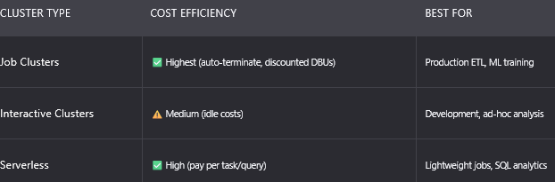
2. Instance Selection

Spot Instances: Use for fault-tolerant workloads (60–90% discount).
Photon: Reduces runtime → lowers cost.
Right-Sizing: Monitor Spark UI for CPU/memory underutilization.

3. Auto Termination

Set 15–30 mins for interactive clusters.
Enforce via Cluster Policies.

B. Storage Optimization

1. Delta Lake Maintenance

OPTIMIZE: Merge small files → reduce metadata overhead.
Z-ORDER: Reduce I/O for filtered queries.
VACUUM: Delete old files (default 7-day retention).

2. Tiered Storage

Move cold data to low-cost tiers (S3 Glacier, Azure Cool Blob).

C. Licensing (DBU) Management

DBU Types & Pricing

Monitoring

Use Account Console → Usage to track:
DBUs by workspace, user, workload
Cost per query (SQL)
Set budget alerts via cloud provider.

D. Operational Best Practices

Use Workflows instead of notebooks for production.
Schedule non-critical jobs during off-peak hours (better spot availability).
Disable public cluster access to prevent data egress costs.
Use Unity Catalog to avoid redundant data copies.

30. What is the Databricks SQL analytics offering?

Databricks SQL is a serverless, high-performance SQL warehouse built for BI, dashboards, and ad-hoc analytics — with seamless integration into the Lakehouse. Core Components are

1. SQL Warehouses (Compute)

Serverless Option: No cluster management; auto-scales per query.
Provisioned Option: Pre-warmed clusters for consistent latency.
Photon-Powered: All queries run on Photon engine (3–10x faster).

2. SQL Editor & Dashboards

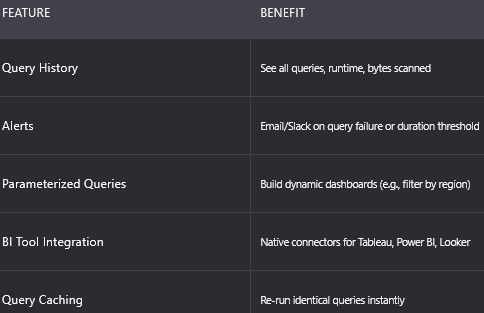
Web-based SQL IDE: With autocomplete, query history, and explain plans.
Interactive Dashboards: Build visualizations (charts, tables) with filters.
Scheduled Refresh: Dashboards auto-update (e.g., hourly).

3. Query Federation

Query external sources without ETL:
Snowflake, Redshift, BigQuery, SQL Server
Via Databricks SQL Connectors

4. Governance & Security

Unity Catalog Integration:
Row/column-level security
Audit logs
Data lineage
SSO & SCIM: Enterprise identity management.

Use Cases

Business Analysts: Self-serve SQL on Delta Lake tables.
Dashboards: Real-time sales, marketing, or ops metrics.
Data Exploration: Ad-hoc queries on petabyte-scale data.
Data Sharing: Expose curated datasets to external partners via Delta Sharing.

31. What is Structured Streaming in Databricks?

Structured Streaming is Apache Spark’s high-level API for processing real-time data streams as unbounded tables that are continuously updated. In Databricks, it is deeply integrated with Delta Lake, enabling exactly-once processing, stateful computations, and unified batch/stream pipelines.

Unlike legacy streaming systems (e.g., Spark Streaming with DStreams), Structured Streaming uses the same DataFrame/Dataset API as batch processing — making it declarative, fault-tolerant, and easy to reason about. Key architectural principles are

1. Continuous Micro-Batch Execution (Default Mode)

Data is ingested in small micro-batches (e.g., every 1–10 seconds).
Each batch is processed as a static DataFrame using the same Catalyst optimizer as batch jobs.
Checkpointing: Maintains offsets (source position) and state (e.g., window aggregates) in cloud storage for fault tolerance.

2. Continuous Processing Mode (Low-Latency)

Sub-second latency (<100ms).
Only supports simple operations (e.g., map, filter).
Not widely used in production due to limited operator support.

3. Event-Time Processing & Watermarks

Handles out-of-order and late-arriving data using event-time semantics.
Watermark: A threshold (e.g., 10 minutes) beyond which late data is discarded.

windowed = df \
  .withWatermark("event_time", "10 minutes") \
  .groupBy(window("event_time", "5 minutes"), "user_id") \
  .count()

Databricks-Specific Enhancements

1. Delta Lake as Source and Sink

Source: Read stream from Delta table:

spark.readStream.format("delta").table("raw_events")

Sink: Write stream to Delta table with exactly-once guarantees:

df.writeStream \
  .format("delta") \
  .outputMode("append") \
  .option("checkpointLocation", "/chkpt/events") \
  .table("clean_events")

2. Auto Loader Integration

Ingest cloud files (JSON, CSV, Parquet) as a stream:

spark.readStream \
  .format("cloudFiles") \
  .option("cloudFiles.format", "json") \
  .load("s3://bucket/events/")

3. Delta Live Tables (DLT)

Declarative streaming pipelines:

@dlt.table
def events_stream():
    return spark.readStream.format("cloudFiles").load("/raw")

Same code runs in streaming or batch backfill mode.

4. Exactly-Once Semantics

Guaranteed via:
Idempotent writes to Delta Lake
Offset tracking in checkpoint
Transaction log for ACID compliance

Use Cases

Real-time fraud detection
IoT telemetry monitoring
Clickstream analytics
CDC (Change Data Capture) from databases

32. How is security implemented in Databricks clusters?

Security in Databricks clusters is enforced through isolation, identity propagation, encryption, and network controls; ensuring least-privilege access to data and compute.

Standard Cluster: Single-user; code runs with user’s identity

High Concurrency Cluster: Multi-user; containerized isolation + credential passthrough

Credential Passthrough (Critical for Security)

Purpose: Allow users to access cloud storage (S3, ADLS) using their own IAM/AD credentials — not shared cluster credentials.
How it works:
Azure: Maps Azure AD identity to Azure RBAC on storage.
AWS: Uses IAM roles mapped via SAML federation.
Result: Enforces row/column-level security at the storage layer (e.g., user can only read their department’s data).

Network Security

1. Private Network Deployment

AWS: VPC peering, PrivateLink
Azure: VNet injection, Private Endpoint
GCP: VPC Service Controls
Effect: All traffic stays within cloud provider’s backbone — no public internet exposure.

2. IP Access Lists

Restrict workspace login to corporate IP ranges.
Block public cluster access.

Encryption

Secret Management

Databricks Secrets: Store credentials in scoped backends (Azure Key Vault, AWS Secrets Manager).
Accessed via dbutils.secrets.get()—never exposed in logs.

Audit & Monitoring

Cluster logs shipped to cloud storage.
Audit logs capture all cluster creation/termination events.
Integration with SIEM tools (Splunk, Datadog).

33. How can you use Databricks to reduce data skew?

Data skew occurs when data is unevenly distributed across partitions — causing some tasks to take much longer than others (“stragglers”). Databricks provides multiple techniques to detect and mitigate skew.

A. Detection

1. Spark UI

Go to Stages tab → look for:
Task duration variance (e.g., 99 tasks at 1s, 1 task at 300s)
Shuffle read/write imbalance

2. Query Profile (Photon)

Visualize skew in join/aggregation keys.

B. Mitigation Techniques

1. Salting (For Aggregations)

Add a random prefix to skewed keys to distribute load:

from pyspark.sql.functions import rand, col

# Add salt to user_id
salted = df.withColumn("salt", (rand() * 10).cast("int"))
salted = salted.withColumn("salted_key", col("user_id") * 10 + col("salt"))

# Aggregate on salted_key
result = salted.groupBy("salted_key").sum("amount")

# Remove salt
final = result.withColumn("user_id", (col("salted_key") / 10).cast("int"))

2. Skew Join Optimization (Automatic in Databricks)

Databricks’ Adaptive Query Execution (AQE) detects skew at runtime:
Splits skewed partitions into smaller tasks.
Broadcasts small skewed keys.
Enabled by default in DBR 10+.

3. Repartitioning

Explicitly repartition on a better key:

df.repartition(200, "country", "device")

4. Broadcast Joins (For Small Tables)

Force broadcast if one table is small:

from pyspark.sql.functions import broadcast
df.join(broadcast(small_df), "key")

5. Z-Ordering (For Filter Skew)

If queries filter on skewed columns (e.g., user_id = 'VIP'), use Z-Ordering to co-locate hot keys.

C. Prevention

Data modeling: Avoid high-cardinality keys with extreme distributions.
Monitoring: Set alerts on task duration variance.

34. How do you handle schema drift in Databricks?

Schema drift occurs when the structure of incoming data changes over time (e.g., new columns, type changes). Databricks handles this via Delta Lake’s schema evolution and Auto Loader’s schema inference.

A. Delta Lake Schema Evolution

1. Schema Enforcement (Default)

Rejects writes that don’t match the table schema — prevents bad data.

2. Schema Evolution (Opt-in)

Use mergeSchema = true to add new columns:

df.write \
  .format("delta") \
  .mode("append") \
  .option("mergeSchema", "true") \
  .save("/table")

Supported changes:
✅ Add columns
✅ Change nullability
⚠️ Limited type widening (e.g., INT → BIGINT)
❌ Rename/drop columns (use REPLACE WHERE or recreate)

3. Backward Compatibility

Old records show NULL for new columns.
Existing queries continue to work.

B. Auto Loader for Streaming Ingestion

Auto Loader automatically handles schema drift in file-based streams:

1. Schema Inference

Infers schema from first batch of files.

2. Schema Evolution

Detects new columns in subsequent files.
Automatically evolves the stream schema (uses mergeSchema under the hood).

3. Schema Registry (Optional)

Store inferred schema in a schema location:

.option("cloudFiles.schemaLocation", "/schema/events")

C. Best Practices

35. How do you use Databricks SQL dashboards?

Databricks SQL Dashboards are interactive, web-based visualizations built on top of SQL queries; enabling self-service analytics for business users.

A. Core Components

1. Queries

Write SQL in the SQL Editor.
Save as query objects with names and descriptions.
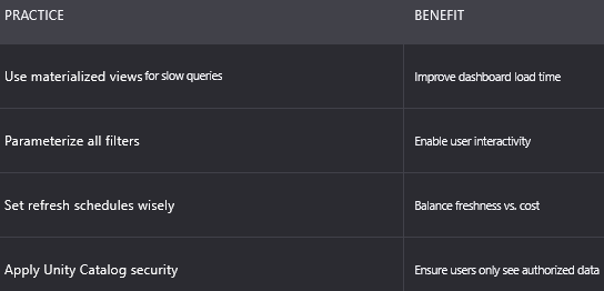
Parameterize using widgets:

SELECT * FROM sales WHERE region = '{{region}}'

2. Visualizations

Chart types: Bar, line, pie, scatter, table, map.
Customization: Colors, axes, legends, tooltips.
Filters: Add dashboard-level filters (e.g., date range).

3. Dashboard Layout

Drag-and-drop tiles (queries) onto canvas.
Resize and arrange for optimal storytelling.

B. Advanced Features

1. Scheduled Refresh

Set refresh frequency (e.g., hourly, daily).
Ensures dashboards show up-to-date data.

2. Alerts

Trigger email/Slack notifications when:
Query result exceeds threshold (e.g., error_rate > 0.05)
Query fails

3. Sharing & Permissions

Share dashboards with:
Workspace users
External users (via Delta Sharing)
Unity Catalog: Apply row/column security to underlying tables.

4. Embedding

Embed dashboards in internal portals via iframe (with SSO).

C. Use Case Workflow

Data Engineer: Creates Delta table sales_daily.

Analyst:

Writes SQL query: SELECT region, SUM(revenue) FROM sales_daily GROUP BY region
Adds bar chart visualization
Creates dashboard “Sales Performance”
Adds parameter {{date}} for dynamic filtering

Manager:

Views dashboard in browser
Selects date = '2024-06-01'
Sees real-time sales by region

D. Best Practices

36. What are Delta tables and how to optimize them?

A Delta table is a transactional storage layer built on top of Apache Parquet, enhanced with a transaction log (_delta_log) to provide ACID compliance, time travel, schema enforcement, and unified batch/streaming access. It is the default table format in Databricks and the foundation of the Lakehouse architecture. Core Components are

Data Files: Stored in Parquet format in cloud object storage (S3, ADLS, GCS).

Transaction Log: A hidden directory _delta_log containing:

JSON files: Record every write, delete, update, or schema change as an atomic transaction.
Checkpoint files (Parquet): Compact every 10 commits for fast metadata reads.

Metadata: Table schema, partitioning info, and file statistics (min/max values per column).

Optimization in a delta table mainly focuses on query performance, storage efficiency, and metadata scalability.

1. File Compaction (OPTIMIZE)

Problem: Small files → high metadata overhead → slow queries.
Solution: Merge small files into larger ones (e.g., 1 GB):

OPTIMIZE events_table;

Best Practice: Run during off-peak hours; target file size = 1 GB.

2. Z-Ordering (Multi-Column Clustering)

Problem: Queries filter on multiple columns (e.g., country, device) → scan many files.
Solution: Physically co-locate related data using a Z-order curve:

OPTIMIZE events_table ZORDER BY (country, device, event_type);

Impact: Reduces I/O by 90%+ for multi-predicate queries.
Limitation: Avoid >4 columns; re-run after large data loads.

3. Partitioning

Use Case: High-cardinality, low-selectivity columns (e.g., date, region).

CREATE TABLE events (
  event_time TIMESTAMP,
  user_id BIGINT,
  ...
) USING DELTA
PARTITIONED BY (DATE(event_time));

Anti-Pattern: Over-partitioning (e.g., by user_id) → too many small partitions.

4. Vacuum Old Files

Delta retains old files for time travel (default: 7 days).
Free up storage:

VACUUM events_table RETAIN 168 HOURS; -- 7 days

VACUUM is irreversible. It ensures no active time-travel queries.

5. Data Skipping

Automatic: Uses min/max statistics in Parquet footers + Delta log.
Enhance: Ensure columns used in filters have good cardinality and non-null values.

6. Caching (Delta Cache)

Automatic: Hot data cached in cluster SSDs.
Manual: Cache frequently accessed tables:

spark.sql("CACHE TABLE events");

7. Monitoring Optimization

Use DESCRIBE DETAIL table to check:

numFiles
sizeInBytes
partitionColumns

Track files read per query in Spark UI.

37. What is Delta Sharing

Delta Sharing is an open protocol for secure, real-time data sharing across organizations — without copying data or requiring recipients to use Databricks. It enables “data as a product” by allowing providers to share live Delta tables with external consumers via REST APIs. Here is how it works

1. Architecture

Provider: Databricks workspace with Unity Catalog.
Recipient: Any system with a Delta Sharing connector (Databricks, Power BI, Tableau, Python, etc.).
Protocol: Open, REST-based, with signed URLs for secure file access.

2. Sharing Workflow

Provider creates a share:

CREATE SHARE sales_share;
ALTER SHARE sales_share ADD TABLE sales;

2. Grants access to recipient (via email or Databricks account):

GRANT SELECT ON SHARE sales_share TO RECIPIENT partner_a;

3. Recipient accesses data:

In Databricks: CREATE TABLE sales USING deltaSharing LOCATION '...';
In Python: pd.read_delta_sharing("https://...")

3. Security & Governance

Zero Data Copy: Recipient reads directly from provider’s cloud storage.
Fine-Grained Access: Share entire tables or row/column-filtered views.
Audit Logs: Track who accessed what and when.
Revocation: Instantly revoke access — no data left behind.

Use Cases

Cross-company collaboration: Share customer data with partners.
Regulatory reporting: Provide auditors live access.
Monetization: Sell data products via API.

38. What are best practices for debugging Spark jobs in Databricks?

Debugging Spark jobs requires a systematic approach leveraging Databricks’ built-in tooling.

A. Use the Spark UI (Primary Tool)

Access via notebook → “View” → “Spark UI” or job run details.

Key Tabs

Jobs: See DAG, stage duration, task distribution.
Stages: Identify stragglers, skew, GC overhead.
Storage: Check if RDDs/DataFrames are cached.
SQL: View physical plans for DataFrame operations.

Diagnose Common Issues

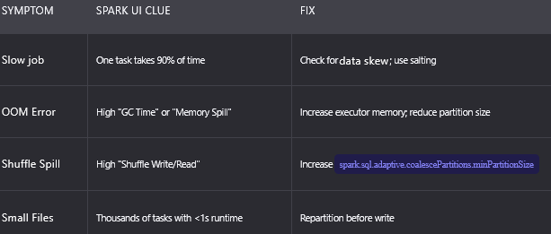
B. Logging & Print Statements

Avoid .show() in production (triggers job).
Use .explain() to see plan without execution:

df.filter(...).explain("extended")

Log intermediate counts:

print(f"Rows after filter: {df.count()}")

C. Delta Lake-Specific Debugging

DESCRIBE HISTORY table: See operation type, user, and schema changes.
DESCRIBE DETAIL table: View file stats, partitioning, size.
Time Travel: Reproduce issues on historical versions:

SELECT * FROM table VERSION AS OF 10;

D. Cluster Configuration Checks

Executor Memory: Too low → OOM; too high → underutilization.
Cores per Executor: 2–5 cores optimal (avoid 1 core).
Dynamic Allocation: Enable for variable workloads.

E. Photon-Specific Debugging (Databricks SQL)

Use Query Profile to see:
CPU time per operator
I/O wait time
Data skipping effectiveness

39. How would you optimize a spark job running on Databricks?

Optimization is iterative and covers compute, I/O, memory, and query logic.

Step 1: Profile the Job

Run job → open Spark UI → identify bottlenecks:
Longest stage
Skewed tasks
Shuffle spill

Step 2: Optimize Data Layout

Source Data:

Use Delta tables with Z-ORDER on filter columns.
Ensure partitioning aligns with query patterns.

Intermediate Data:

Cache hot DataFrames: df.cache().count()
Repartition before shuffles: df.repartition(200, "key")

Step 3: Tune Spark Configuration

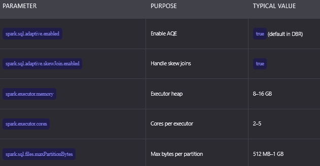
Step 4: Optimize Query Logic

Filter Early: Push filters to source (predicate pushdown).
Select Only Needed Columns: Avoid SELECT *.
Broadcast Small Tables:

df.join(broadcast(small_df), "key")

Avoid UDFs: Use built-in functions (e.g., regexp_extract vs. Python UDF).

Step 5: Leverage Databricks-Specific Features

Photon: Ensure job runs on Photon (DBR 10+).
Delta Cache: Hot data automatically cached in SSDs.
Serverless: For lightweight jobs, use Serverless Compute (faster startup).

Step 6: Monitor & Iterate

Track job duration, cost, and files read over time.
Use Databricks Query History (SQL) or Job Run Metrics.

40. How to use MLflow in Databricks?

MLflow is Databricks’ native MLOps platform; fully integrated into the Lakehouse for experiment tracking, model registry, and deployment.

A. MLflow Tracking (Experiment Management)

1. Automatic Logging

Every notebook run auto-logs:
Parameters (e.g., learning_rate)
Metrics (e.g., accuracy)
Source code (Git commit)
Spark UI link
View in Experiments sidebar.

2. Manual Logging

import mlflow
mlflow.log_param("max_depth", 5)
mlflow.log_metric("rmse", 0.85)
mlflow.log_artifact("model.pkl")

3. Compare Runs

Select multiple runs → visualize metric trends, parameter diffs.

B. MLflow Models (Packaging)

1. Log Model

mlflow.sklearn.log_model(model, "model")

saves model with:

Code (predict() function)
Dependencies (conda.yaml)
Multiple flavors (Python, PyTorch, etc.)

2. Load Model

model = mlflow.pyfunc.load_model("runs:/<run_id>/model")

C. MLflow Model Registry (Governance)

1. Register Model

mlflow.register_model("runs:/<run_id>/model", "fraud_detection")

2. Lifecycle Stages

None → Staging → Production
Add descriptions, tags, and aliases.

3. Unity Catalog Integration

Models appear as first-class objects in Unity Catalog.
Apply row/column security and lineage tracking.

D. Model Serving (Deployment)

1. Real-Time Endpoints

Deploy model as REST API:

workspace.model_serving.create_endpoint(
  name="fraud-api",
  config=...
)

Features:

Auto-scaling
A/B testing
Monitoring (latency, error rate)

2. Batch Inference

Use Databricks Workflows to run batch predictions:

spark.read.table("new_data") \
  .withColumn("prediction", predict_udf("features")) \
  .write.saveAsTable("predictions")

E. Advanced Features

1. AutoML

Point-and-click UI to auto-train models.
Generates Python notebook with full MLflow tracking.

2. Feature Store

Central catalog of curated features.
Ensures training-serving consistency.

3. LLM Support (MLflow 2.10+)

Track prompt templates, LLM parameters, and evaluation metrics (toxicity, relevance).

F. CI/CD Integration

Promote models via webhooks:

# On PR merge → promote to Production
client.transition_model_version_stage(
  name="fraud_detection",
  version=5,
  stage="Production"
)

41. How is Databricks integrated with orchestration tools?

Databricks provides native and third-party integrations with leading orchestration tools to enable end-to-end pipeline automation, dependency management, and CI/CD.

A. Native Orchestration: Databricks Workflows (Jobs)

Databricks Workflows is the built-in orchestration service for scheduling and managing data and ML pipelines. Key capabilities are

Multi-Task DAGs: Define dependencies between notebooks, Python scripts, Delta Live Tables, or JARs.
Triggers: Cron schedules, manual runs, or API/webhook triggers.
Compute Isolation: Each task runs on a dedicated job cluster (auto-terminated).
Parameterization: Pass parameters to tasks (e.g., {"env": "prod"}).
Notifications: Email, Slack, or webhook alerts on success/failure.
Monitoring: Full run history with logs, Spark UI, and cost tracking

B. Third-Party Orchestration Integrations

1. Apache Airflow

Databricks Operator: Submit jobs via DatabricksSubmitRunOperator.
Workflow:

from airflow.providers.databricks.operators.databricks import DatabricksSubmitRunOperator

submit_job = DatabricksSubmitRunOperator(
    task_id="run_etl",
    json={
        "notebook_task": {"notebook_path": "/ETL/main"},
        "new_cluster": { ... }
    }
)

Use Case: When Airflow is the central orchestrator for hybrid (cloud + on-prem) workflows.

2. Azure Data Factory (ADF)

Databricks Activity: Trigger notebooks or JARs in Azure Databricks.
Linked Service: Authenticates via Azure AD or personal access token.
Parameter Passing: Map ADF pipeline variables to notebook widgets.

3. AWS Step Functions

Databricks Job Task: Invoke Databricks jobs via REST API.
Error Handling: Retry policies and fallback states.

4. Prefect, Dagster, Kubeflow

Use Databricks REST API or CLI within task definitions.
Example (Prefect):

from prefect import task
import subprocess

@task
def run_databricks_job():
    subprocess.run(["databricks", "jobs", "run-now", "--job-id", "123"])

C. CI/CD Integration

Git (via Repos): Store notebooks in GitHub/GitLab; trigger jobs on PR merge.
Terraform: Deploy Databricks resources (clusters, jobs, permissions) as code.
Databricks CLI: Automate job deployment in CI pipelines:

databricks jobs create --json-file job-config.json
databricks jobs run-now --job-id $(cat job-id.txt)

D. Event-Driven Orchestration

Cloud Events: Trigger Databricks jobs via:
AWS EventBridge → Lambda → Databricks REST API
Azure Event Grid → Function App → Databricks API

Use Case: Ingest new file → trigger ETL job.

42. How does autoscaling work in Databricks clusters?

Autoscaling dynamically adjusts the number of worker nodes in a cluster based on workload demand, optimizing cost and performance.

A. Types of Autoscaling

1. Standard Autoscaling (All-Purpose Clusters)

Scale-Out: Add workers when tasks are backlogged (e.g., >2 tasks per core).
Scale-In: Remove idle workers after stable low utilization (default: 10 mins).
Bounds: Defined by min/max workers (e.g., 2–20 nodes).

2. Optimized Autoscaling (Job Clusters)

Faster Scale-Out: Adds workers in parallel (not sequentially).
Aggressive Scale-In: Removes idle workers after 1–2 mins.
Spot Instance Handling: Automatically replaces preempted spot instances.

B. Technical Mechanics

1. Metrics Used

Task Queue Length: Number of pending tasks.
CPU Utilization: Per-worker core usage.
Shuffle Pressure: Data spill to disk.

2. Scaling Logic

Scale-Out Condition:

Pending Tasks > (Active Cores * 2)

Scale-In Condition:

CPU Utilization < 20% for 10 minutes (standard) or 1–2 mins (job clusters)

3. Instance Pools Integration

Pull pre-warmed instances from pool → near-instant scale-out.

C. Configuration Best Practices

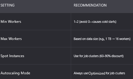
D. Monitoring Autoscaling

Cluster Event Log: Shows scale-out/in events.
Spark UI: Track task scheduling delays.
Cloud Metrics: Monitor VM utilization (AWS CloudWatch, Azure Monitor).

43. How do you monitor Databricks cluster and job health?

Monitoring in Databricks combines built-in UIs, logs, metrics and alerts for proactive operations.

A. Cluster Monitoring

1. Cluster Event Log

Location: Cluster → Event Log tab.
Shows:
Node additions/removals
Driver/executor logs
Autoscaling decisions

2. Spark UI

Access: Notebook → View → Spark UI.
Key Metrics:
Stages: Task duration, skew, GC time
Executors: Memory/CPU usage, disk spill
SQL: Physical plan, data skipping

3. System Metrics

Databricks System Tables (Unity Catalog):

SELECT * FROM system.compute.clusters;
SELECT * FROM system.compute.cluster_events;

Cloud Metrics: Export to CloudWatch, Azure Monitor, or Datadog.

B. Job Monitoring

1. Job Run History

Location: Workflows → Job → Runs.
Shows:
Start/end time
Parameters
Logs (stdout/stderr)
Spark UI link

2. Alerts & Notifications

Configure on:

Failure
Duration > threshold
Success (for critical jobs)
Channels: Email, Slack, webhook.

3. Query History (SQL)

Location: SQL → Query History.
Metrics: Runtime, bytes scanned, warehouse used.

C. Advanced Monitoring

1. Audit Logs

Content: User logins, cluster creation, permission changes.
Export: To S3/ADLS for SIEM integration (Splunk, Datadog).

2. Unity Catalog System Tables

Monitor data access, lineage, and storage usage:

SELECT * FROM system.access.table_lineage;
SELECT * FROM system.storage.table_storage_history;

3. Custom Dashboards

Build in Databricks SQL or Power BI using system tables.

44. Explain Delta Live Tables.

Delta Live Tables (DLT) is Databricks’ declarative framework for building reliable, testable, and maintainable data pipelines that work identically for batch and streaming. Core principles are:

Declarative: Define what the pipeline should do — not how to do it.

Unified: Same code runs in continuous streaming or batch backfill mode.

Reliable: Built-in data quality enforcement and dependency resolution.

Observable: Auto-generated DAG, metrics, and data lineage.

Technical Implementation

1. Declarative Syntax (Python Example)

import dlt

@dlt.table
def sales_raw():
    return (
        spark.readStream  # or spark.read for batch
          .format("cloudFiles")
          .option("cloudFiles.format", "json")
          .load("/raw/sales")
    )

@dlt.table
@dlt.expect("valid_amount", "amount > 0")
def sales_clean():
    return dlt.read("sales_raw").filter(col("status") == "success")

2. Automatic Orchestration

DLT infers dependencies from dlt.read() calls.
Builds a visual DAG in the UI.

3. Data Quality Enforcement

@dlt.expect: Drop rows that violate condition.
@dlt.expect_or_fail: Fail entire pipeline on violation.
Metrics: Track % of dropped rows per rule.

4. Deployment Modes

Continuous: Real-time streaming.
Triggered: Batch backfill (e.g., reprocess last 30 days).

Key Benefits

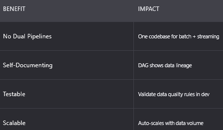
45. Explain event-driven processing in Databricks.

Event-driven processing executes pipelines in response to events (e.g., new file arrival, database change) rather than on a fixed schedule. The core components are

1. Event Sources

Cloud Storage Events:
AWS: S3 Event Notifications → SQS/SNS
Azure: Blob Storage Events → Event Grid
GCP: Cloud Storage Notifications → Pub/Sub
Database CDC: Debezium → Kafka → Databricks
Application Events: Custom apps → Kafka/Pub/Sub

2. Event Ingestion

Auto Loader: Native Databricks service for file-based events:

spark.readStream.format("cloudFiles").load("s3://bucket/")

Kafka Connector: For message-based events:

spark.readStream.format("kafka").option("kafka.bootstrap.servers", "...").load()

3. Processing Engine

Structured Streaming: Process events in micro-batches.
Delta Live Tables: Declarative event-driven pipelines.

4. Triggering Downstream Actions

Write to Delta Table → trigger materialized view refresh.
Call REST API (e.g., send alert via Slack webhook).
Invoke Databricks Job via REST API.

B. Workflow Example

Event: New JSON file lands in S3.
Ingestion: Auto Loader detects file → streams to Delta table raw_events.
Processing: DLT pipeline cleans/enriches data → writes to clean_events.
Action:

Real-time: Dashboard updates via Databricks SQL.
Batch: Nightly job aggregates data for ML training.

C. Advantages Over Scheduled Processing

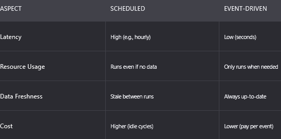
46. Explain cluster policies in Databricks?

Cluster Policies are centralized, administrator-defined rules that enforce governance, security, and cost controls on cluster configurations in Databricks. They allow admins to restrict or preset cluster attributes (e.g., instance types, auto-termination, runtime versions) while still giving users flexibility to create clusters within approved boundaries. Core purpose and benefits are

Cost Control: Enforce use of spot instances, max cluster size, auto-termination

Security: Disable public IP access, enforce FIPS compliance, restrict runtimes

Compliance: Mandate encryption, VPC/VNet placement, runtime versions

Standardization: Ensure consistent cluster configurations across teams

Self-Service: Empower users to create clusters — without violating governance

Technical Implementation

1. Policy Attributes

Policies define allowed values or fixed values for cluster settings using JSON:

{
  "spark_version": {
    "type": "fixed",
    "value": "13.3.x-scala2.12"
  },
  "node_type_id": {
    "type": "allowlist",
    "values": ["i3.xlarge", "r5d.2xlarge"]
  },
  "autotermination_minutes": {
    "type": "range",
    "minValue": 10,
    "maxValue": 60
  },
  "enable_elastic_disk": {
    "type": "fixed",
    "value": true
  },
  "aws_attributes.availability": {
    "type": "fixed",
    "value": "SPOT"
  }
}

2. Policy Types

Fixed: User cannot change (e.g., spark_version).
Allowlist: User selects from predefined options (e.g., instance types).
Blocklist: Prevent specific values (e.g., block m5.large).
Range: Numeric bounds (e.g., autotermination_minutes: 10–60).

3. Assignment & Inheritance

Policies are assigned to users, groups, or service principals.
A user can have multiple policies — the most permissive applies.
Admins bypass policies (unless restricted via account settings).

Common Enterprise Use Cases

Data Science Team: Allow GPU instances; max 8 workers; auto-terminate in 30 mins

Production ETL: Enforce job clusters with spot instances; DBR 13.3 LTS; no public IP

Regulated Workloads: Require FIPS-enabled runtime; VPC placement; CMK encryption

Cost-Sensitive Dev: Max cluster cost = $5/hr; only spot instances; auto-terminate in 15 mins

Best Practices

Start restrictive, then relax as needed.
Use naming conventions (e.g., prod-etl-policy, ds-gpu-policy).
Combine with Unity Catalog for end-to-end governance.
Audit policy usage via system tables:

SELECT * FROM system.compute.cluster_policies;

47. What is Structured Streaming checkpointing?

Checkpointing in Structured Streaming is the mechanism by which Spark persistently stores metadata about a streaming query’s progress — including input offsets, aggregation state, and sink commit history — to enable fault tolerance and exactly-once processing.

Without checkpointing, a failed job would reprocess all data from the beginning, causing duplicates or data loss.

What Is Stored in the Checkpoint Location?

The checkpoint directory (e.g., s3://bucket/checkpoints/sales/) contains:

Offsets:

Tracks how much data has been read from each source partition (e.g., Kafka topic partition, file directory).

Stored in offsets/ subdirectory as JSON.

Commit Logs:

Records which batches have been successfully written to the sink.
Prevents reprocessing on restart.

State Store:

For stateful operations (e.g., groupBy, window), stores aggregation state (e.g., running counts).
Uses RocksDB (on local disk) or cloud storage (for cloud-native state).

Source Metadata:

Schema, partition info, and custom source state.

How Checkpointing Enables Fault Tolerance

Job Failure: Cluster crashes during batch 10.
Restart: Spark reads offsets/ to resume from batch 10 (not 0).
Exactly-Once: Commit logs ensure batch 10 is not reprocessed if already written.
State Recovery: Aggregation state (e.g., window counts) is restored from state store.

Configuration in Databricks

df.writeStream \
  .format("delta") \
  .outputMode("append") \
  .option("checkpointLocation", "s3://my-bucket/checkpoints/sales") \
  .table("sales_stream")

Best Practices are

Unique checkpoint path per query (avoid conflicts).
Do not delete checkpoint data — breaks exactly-once guarantees.
Monitor checkpoint size: Large state → high storage cost.
Use Delta Lake as sink: Combines checkpointing with ACID transactions for end-to-end exactly-once.

48. How to monitor job failures and cluster health?

Monitoring in Databricks combines built-in UIs, system tables, logs, and alerts for proactive operations.

A. Job Failure Monitoring

1. Job Run History (Primary Tool)

Location: Workflows → Job → Runs.
Key Details:
Error message (with line number for notebooks)
Logs (stdout/stderr)
Spark UI link for detailed diagnostics
Parameters used in the run

2. Alerts & Notifications

Configure per job:
On failure: Email, Slack, or webhook.
On success (for critical jobs).
On duration > threshold (e.g., >1 hour).

3. System Tables (Unity Catalog)

Query job history programmatically:

SELECT * FROM system.job_runs 
WHERE status = 'FAILED' 
  AND start_time > current_date() - INTERVAL 7 DAYS;

4. Audit Logs

Track job creation/deletion:

SELECT * FROM system.access.audit 
WHERE service_name = 'jobs' AND action_name = 'runNow';

B. Cluster Health Monitoring

1. Cluster Event Log

Location: Cluster → Event Log tab.
Shows:
Node launch/termination
Driver/executor logs
Autoscaling decisions
Spot instance preemptions

2. Spark UI

Access: Notebook → View → Spark UI.
Diagnose:
Task skew: One task takes 90% of time
OOM errors: High GC time or memory spill
Shuffle pressure: Large shuffle read/write

3. System Metrics

Databricks System Tables:

-- Cluster utilization
SELECT cluster_id, avg(utilization) 
FROM system.compute.cluster_utilization 
GROUP BY cluster_id;

-- Spot preemption rate
SELECT count(*) 
FROM system.compute.cluster_events 
WHERE details LIKE '%PREEMPTED%';

4. Cloud Monitoring

Export metrics to:
AWS CloudWatch
Azure Monitor
Datadog/Splunk (via log shipping)

C. Proactive Alerting Strategy

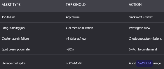
49. What integration possibilities does Databricks support?

Databricks offers deep, native integrations across the modern data and AI stack; enabling end-to-end workflows without vendor lock-in.

A. Cloud Platforms

AWS: S3, IAM, Glue, Kinesis, Redshift, SageMaker, EventBridge

Azure: ADLS, Azure AD, Synapse, Event Hubs, Purview, Key Vault

GCP: GCS, BigQuery, Pub/Sub, Vertex AI, Secret Manager

B. Data Sources & Sinks

Databases: JDBC/ODBC to Snowflake, Oracle, SQL Server, PostgreSQL.
Streaming: Kafka, Kinesis, Event Hubs (via Auto Loader or connectors).
File Formats: Parquet, CSV, JSON, Avro, ORC, Delta.
BI Tools: Tableau, Power BI, Looker (via Databricks SQL endpoint).

C. DevOps & CI/CD

Git: GitHub, GitLab, Azure DevOps, Bitbucket (via Repos).
IaC: Terraform, ARM, CloudFormation.
CI/CD: Jenkins, GitHub Actions, Azure DevOps Pipelines.
Package Management: PyPI, Conda, Maven.

D. ML & AI Ecosystem

MLOps: MLflow (native), SageMaker, Vertex AI

Frameworks: TensorFlow, PyTorch, scikit-learn, XGBoost

LLMs: Hugging Face, LangChain, LlamaIndex, Databricks Foundation Models

Vector DBs: Pinecone, Weaviate, Qdrant, FAISS

E. Security & Governance

Secrets: Azure Key Vault, AWS Secrets Manager, HashiCorp Vault.
IAM: SAML, SCIM, Okta, Azure AD, Ping Identity.
Data Governance: Unity Catalog (unified), Apache Atlas (legacy).

F. Monitoring & Observability

Logs: Ship to Splunk, Datadog, ELK, Sumo Logic.
Metrics: Prometheus, Grafana, CloudWatch, Azure Monitor.
Alerting: Slack, PagerDuty, email, webhooks.

G. Partner Ecosystem

ETL: Fivetran, Stitch, Talend, Informatica.
Data Quality: Great Expectations, Soda Core, Monte Carlo.
Reverse ETL: Census, Hightouch, SeekWell.

50. How would you optimize a Spark job that is failing or slow?

Optimization is a structured, iterative process combining diagnosis, tuning, and validation.

Step 1: Diagnose the Root Cause

A. For Failing Jobs

Check error logs:
OOM: Increase executor memory; reduce partition size.
ClassNotFound: Add missing JAR/library.
Permission denied: Fix IAM/AD roles or secrets.
Reproduce locally: Run on small dataset in notebook.

B. For Slow Jobs

Open Spark UI → Stages tab:
Skew: One task >> others → use salting or AQE.
Shuffle spill: Increase spark.sql.adaptive.coalescePartitions.minPartitionSize.
Small files: Repartition before write.

Step 2: Optimize Data Layout

Source scan slow: Use Delta tables with Z-ORDER on filter columns

Join slow: Broadcast small table; use AQE skew join

Aggregation slow: Salt skewed keys; increase parallelism

Step 3: Tune Spark Configuration

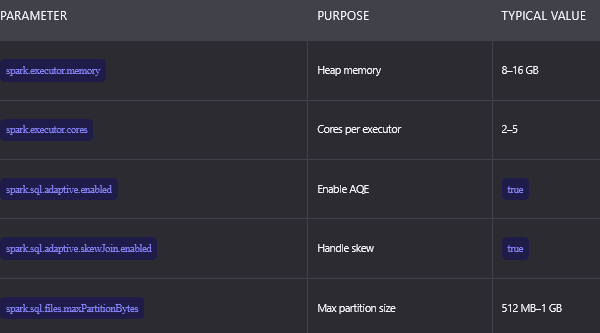
Step 4: Optimize Query Logic

Filter early: Push predicates to source.
Select only needed columns: Avoid SELECT *.
Avoid UDFs: Use built-in functions (e.g., regexp_extract).
Cache hot DataFrames: df.cache().count().

Step 5: Leverage Databricks-Specific Features

Photon: Ensure job runs on DBR 10+ (faster execution).
Delta Cache: Hot data cached in SSDs (automatic).
Serverless: For lightweight jobs, use Serverless Compute.
Instance Pools: Reduce startup time for frequent jobs.

Step 6: Validate & Monitor

Measure before/after: Runtime, cost, files read.
Set up alerts: For regressions in future runs.
Document changes: In Git (via Repos) for reproducibility.

Ace your databricks interview with expertly curated questions and in-depth, practical answers; covering everything from core Spark concepts to advanced Lakehouse architecture, performance optimization, security, and real-world implementation strategies.

1. What is Databricks and how it is not same as Apache Spark?

Key Differences Between Databricks and Apache Spark:

2. Explain the Delta Lake architecture in Databricks

Core Design Principles

Architectural Components

1. Data Files (Parquet)

2. Transaction Log (_delta_log)

3. ACID Transactions

4. Optimizations

5. Time Travel (Versioning)

6. Streaming Integration

3. List the advantages of Delta Lake over traditional data lake and data warehouse?

4. What is new from Databricks Runtime 15 and what are it’s Latest Features?

1. Photon Engine 3.0

2. Serverless Compute

3. Delta Lake 3.0 Integration

4. AI & Generative AI Enhancements

5. Unity Catalog Upgrades

6. Delta Live Tables (DLT) Improvements

7. Language & Library Support

8. Security & Compliance

5. Explain Delta Lakes schema evolution capability.

Schema Evolution Workongs

1. Schema Enforcement (Default Behavior)

2. Enabling Schema Evolution

3. Supported Schema Changes

4. Backward & Forward Compatibility

5. Real-World Example

6. Best Practices

6. How is security managed in Databricks at the workspace and cluster level?

A. Workspace-Level Security

1. Identity & Access Management (IAM)

2. Role-Based Access Control (RBAC)

3. Network Security

4. Audit Logging & Monitoring

B. Cluster-Level Security

1. Cluster Access Control

2. Credential Passthrough (High Concurrency Clusters)

3. Secure Secret Management

4. Isolation & Sandboxing

5. Encryption

7. Explain Unity Catalog and its role.

Core Architecture

Key Capabilities

1. Fine-Grained Access Control

2. Row-Level Security (RLS)

3. Data Lineage & Impact Analysis

4. Audit & Compliance

5. Cross-Cloud & Cross-Workspace Sharing

6. Unified Metadata

8. What is the purpose of Databricks Repos?

Key Features & Workflow

1. Git Integration

2. Notebook-as-Code

3. Branching & Merging

4. CI/CD Integration

5. Collaboration & Audit

9. How does Databricks support multi-cloud and hybrid cloud deployments?

A. Multi-Cloud Support

B. Hybrid Cloud (On-Prem + Cloud)

1. Databricks on AWS/Azure with On-Prem Data Sources

2. Delta Sharing for Hybrid

3. Limited On-Prem Option

C. Multi-Region & Disaster Recovery

10. Describe ML pipelines and MLflow in Databricks.

A. MLflow: The Open MLOps Platform

1. MLflow Tracking

2. MLflow Models

3. MLflow Model Registry

4. MLflow Projects

B. ML Pipelines in Databricks

1. AutoML

2. Feature Store

3. Model Serving

4. Workflows (Jobs) for Orchestration

5. LLM & Generative AI Support

11. What is the difference between a Databricks cluster and a pool?

Instance Pool Features

2. Transaction Log (`_delta_log`)